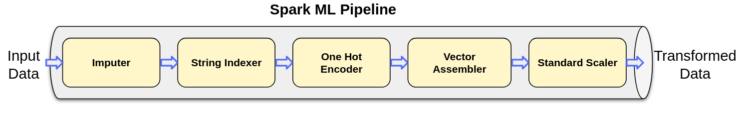
Figure 1: Spark ML pipeline with multiple transformations
This post shows the usage of Spark ML pipelines to transform the data and train the models.
Spark ML pipelines consist of multiple stages which will be run in specific order. These stages can be either Transformers or Estimators. We can see more details on Spark ML Pipelines here
Auto MPG dataset
We will take the example dataset of measuring fuel efficiency of cars. The original dataset is available here
I have taken this data and pre-processed it a bit to use it easily in this example (adding headers, change column delimiter etc.) This dataset which we will use can be downloaded from here
This data contains features: MPG, Cylinders, Displacement, Horsepower, Weight, Acceleration, Model Year, Origin, Car Name. MPG specifies the fuel efficiency of the car.
Visualizing the data
We can load this data and visualize it either using Python or Tableau. The Tableau view for scatter plots is shown below:
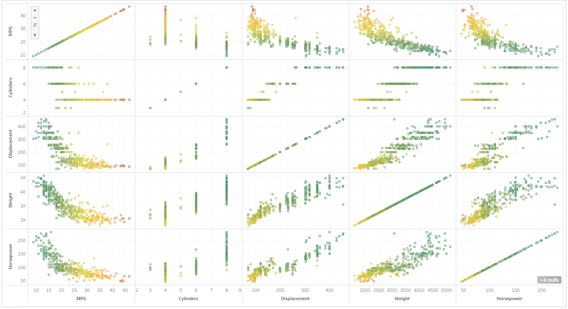
Figure 1: Spark ML pipeline with multiple transformations
The correlation matrix for the features is below:
+------------+------+---------+------------+----------+------+------------+
|            |MPG   |Cylinders|Displacement|Horsepower|Weight|Acceleration|
+------------+------+---------+------------+----------+------+------------+
|MPG         |+1.000|-0.778   |-0.805      |-0.778    |-0.832|+0.423      |
|Cylinders   |-0.778|+1.000   |+0.951      |+0.843    |+0.898|-0.505      |
|Displacement|-0.805|+0.951   |+1.000      |+0.897    |+0.933|-0.544      |
|Horsepower  |-0.778|+0.843   |+0.897      |+1.000    |+0.865|-0.689      |
|Weight      |-0.832|+0.898   |+0.933      |+0.865    |+1.000|-0.417      |
|Acceleration|+0.423|-0.505   |-0.544      |-0.689    |-0.417|+1.000      |
+------------+------+---------+------------+----------+------+------------+
We can see in the scatter plot and correlation matrix that as the horsepower, weight and displacement increase, MPG is reducing.
Reading and transforming the data
Now let us read the data and see the columns, type of columns and more details. To read data, we will use:
spark.read()
	.option("header", true)
        .option("inferSchema", true)
        .option("delimiter", "|")
        .csv("auto-mpg.csv.gz");
We are using these options to read the data:
- • header specifies that there is a header line in the csv file
- • inferSchema to automatically determine the type of data in each column
- • delimiter to sepcify that we are using pipe(‘|’) as the delimiter between the fields
If we print the schema to see the type of each column:
inDs.printSchema();
This shows the output:
root
 |-- MPG: double (nullable = true)
 |-- Cylinders: integer (nullable = true)
 |-- Displacement: double (nullable = true)
 |-- Horsepower: double (nullable = true)
 |-- Weight: double (nullable = true)
 |-- Acceleration: double (nullable = true)
 |-- Model Year: integer (nullable = true)
 |-- Origin: string (nullable = true)
 |-- Car Name: string (nullable = true)
Schema shows that the columns except Origin and Car Name are of numeric type. Let us see the unique values in the Origin column:
inDs.select("Origin").distinct().show();
+------+
|Origin|
+------+
|Europe|
|   USA|
| Japan|
+------+
Origin is a categoric value, we will convert it to one hot encoding.
Similarly car name is also a string feature. Since car name is not having any relation to the fuel efficiency, we will drop this column.
inDs = inDs.drop("Car Name");
Let us see the summary of all the data including the count of values in each column using:
inDs.summary().show();
It shows the below output:
+-------+------------------+------------------+------------------+------------------+-----------------+------------------+------------------+------+
|summary|               MPG|         Cylinders|      Displacement|        Horsepower|           Weight|      Acceleration|        Model Year|Origin|
+-------+------------------+------------------+------------------+------------------+-----------------+------------------+------------------+------+
|  count|               398|               398|               398|               392|              398|               398|               398|   398|
|   mean|23.514572864321615| 5.454773869346734|193.42587939698493|104.46938775510205|2970.424623115578|15.568090452261291| 76.01005025125629|  null|
| stddev| 7.815984312565783|1.7010042445332123|104.26983817119587| 38.49115993282846|846.8417741973268| 2.757688929812676|3.6976266467325862|  null|
|    min|               9.0|                 3|              68.0|              46.0|           1613.0|               8.0|                70|Europe|
|    25%|              17.5|                 4|             104.0|              75.0|           2223.0|              13.8|                73|  null|
|    50%|              23.0|                 4|             146.0|              93.0|           2800.0|              15.5|                76|  null|
|    75%|              29.0|                 8|             262.0|             125.0|           3609.0|              17.2|                79|  null|
|    max|              46.6|                 8|             455.0|             230.0|           5140.0|              24.8|                82|   USA|
+-------+------------------+------------------+------------------+------------------+-----------------+------------------+------------------+------+
We can see that Horsepower has missing values. We will have to fill in those missing values. Also we can note that each feature has different ranges.
We can build the pipeline to transform the data to the required format before we train the models.
Transformer and the purpose of it is summarized below:
Imputer: Since we have missing values in Horsepower column, we will fill the missing data using median of all the remaining values.
StringIndexer: Origin is a categorical column. Before we convert it to a one hot encoding we need to assign label indicies to each unique value. StringIndexer will perform this operation. We can see the assigned values below:
+------+---------+
|Origin|OriginIdx|
+------+---------+
| Japan|      1.0|
|Europe|      2.0|
|   USA|      0.0|
+------+---------+
OneHotEncoder: Once StringIndexer stage is completed, we can convert the categorical values to one-hot encoding using this transformation.
Once this stage completes the transformed categorical value looks like this:
+------+-------------+
|Origin|    OriginVec|
+------+-------------+
|   USA|(2,[0],[1.0])|
| Japan|(2,[1],[1.0])|
|Europe|    (2,[],[])|
+------+-------------+
OriginVec is a sparse vector which shows the nonzero indices and their values. Sparse Vector is an efficient format for this data since at most only one value is set in the vector.
But if we want to see this vector in dense format, we can convert this sparse vector to dense:
transformedDs.select("Origin", "OriginVec")
	.withColumn("OriginVecDense", functions.udf((UDF1<Vector, Object>) Vector::toDense, new VectorUDT())
       		.apply(transformedDs.col("OriginVec"))).distinct().show();
One hot encoded Origin column in sparse and dense format looks like:
+------+-------------+--------------+
|Origin|    OriginVec|OriginVecDense|
+------+-------------+--------------+
| Japan|(2,[1],[1.0])|     [0.0,1.0]|
|   USA|(2,[0],[1.0])|     [1.0,0.0]|
|Europe|    (2,[],[])|     [0.0,0.0]|
+------+-------------+--------------+
VectorAssembler: Vector assembler combines multiple columns into one vector format. We will combine all the transformed columns into one vector.
StandardScaler: The features in the dataset are not in the same range. Machine learning algorithms perform well when data is in similar ranges.
We will use StandarScaler to scale the data.
Build the model, predict and evaluate the model
Once the data is transformed and is ready for training, we can build the model. At first let us split the data and set aside a test data set
Dataset<Row>[] splits = transformedDs.randomSplit(new double[] {0.7, 0.3}, 0);
Dataset<Row> trainDs = splits[0];
Dataset<Row> testDs = splits[1];
First model we will try is a LinearRegression. We can build the model by using:
LinearRegression lr = new LinearRegression()
	.setRegParam(0.3)
	.setFeaturesCol("TrainFeaturesScaled")
	.setLabelCol("MPG");
LinearRegressionModel lrModel = lr.fit(trainDs);
We are setting the train features and the label columns. We are also setting a regularization parameter which will help in better generalization
Once the model is built, we can predict the values of the test data. By default the predicted values are in the column “prediction”. Let us see the 10 predicted values and the expected value.
Dataset<Row> predictions = lrModel.transform(testDs);
predictions.selectExpr("MPG", "round(prediction, 3) as prediction").show(10);
+----+----------+
| MPG|prediction|
+----+----------+
| 9.0|     7.643|
|11.0|    15.812|
|12.0|    11.554|
|13.0|    16.405|
|13.0|    11.631|
|13.0|     12.56|
|13.0|     9.444|
|13.0|     7.372|
|14.0|    14.028|
|14.0|    13.481|
+----+----------+
We can see some of the predictions are close to the actual values. We can quantitatively measure the models performance.
RMSE (Root Mean Squared Error) is a performance measure for regression models. We can measure the RMSE of this model by:
RegressionEvaluator evaluator = new RegressionEvaluator()
	.setLabelCol("MPG")
	.setPredictionCol("prediction")
	.setMetricName("rmse");
This gives us the output:
Linear Regression RMSE on test data = 3.606182319282716
Let us build another model using RandomForestRegressor. This can be done by using:
RandomForestRegressor rfRegressor = new RandomForestRegressor()
	.setNumTrees(8)
	.setSeed(0)
	.setFeaturesCol("TrainFeaturesScaled")
	.setLabelCol("MPG");
RandomForestRegressionModel rfModel = rfRegressor.fit(trainDs);
If we measure the RMSE of this model using the same approach as above, we can see that:
Random Forest Regression RMSE on test data = 2.9796895291729486
This is better performance compared to Linear Regression model.
We can further tweak the model parameters or build different models to further improve the prediction.
Since the goal of this post was to show the usage of Spark ML pipelines and how we can use them to train regression models, we will stop here.