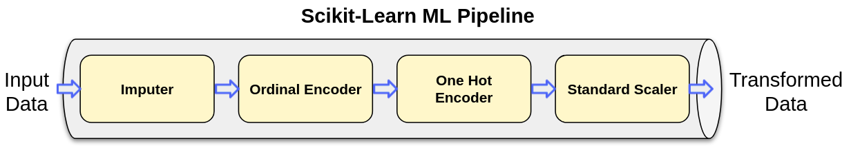
Figure 1: Scikit-Learn ML pipeline with multiple transformations
In this post we will see how we can use Scikit-Learn pipelines to transform the data and train ML models.
Scikit-Learn pipelines can have multiple stages which will be run in specific order. These stages can be either Transformers or Estimators. We can see more details on Scikit-Learn ML Pipelines here.
Auto MPG dataset
We will take the example dataset of measuring fuel efficiency of cars. The original dataset is available here
I have taken this data and pre-processed it a bit to use it easily in this example (adding headers, change column delimiter etc.) This dataset which we will use can be downloaded from here
This data contains features: MPG, Cylinders, Displacement, Horsepower, Weight, Acceleration, Model Year, Origin, Car Name. MPG specifies the fuel efficiency of the car.
Reading the data
To read the data, we will use Pandas library like below:
mpg_data = pd.read_csv('auto-mpg.csv.gz', sep='|')
We can see the details of the loaded data like type of column, count of each field using:
mpg_data.info()
<class 'pandas.core.frame.DataFrame'>
RangeIndex: 398 entries, 0 to 397
Data columns (total 9 columns):
 #   Column        Non-Null Count  Dtype
---  ------        --------------  -----
 0   MPG           398 non-null    float64
 1   Cylinders     398 non-null    int64
 2   Displacement  398 non-null    float64
 3   Horsepower    392 non-null    float64
 4   Weight        398 non-null    float64
 5   Acceleration  398 non-null    float64
 6   Model Year    398 non-null    int64
 7   Origin        398 non-null    object
 8   Car Name      398 non-null    object
dtypes: float64(5), int64(2), object(2)
memory usage: 28.1+ KB
We can see that columns except Origin and Car Name are of numeric type.
Horsepower is missing 6 values. We will fill these values using Imputer.
Origin is a non-numeric column. Let us see the distinct values in the column:
mpg_data['Origin'].unique()
array(['USA', 'Japan', 'Europe'], dtype=object)
Origin is a categorical column. We will convert it to one-hot encoding.
Simlilarly Car Name is a String column. However it does not having any relation with fuel efficiency. We will drop this column.
mpg_data = mpg_data.drop('Car Name', axis=1)
Visualizing the data
Let us visualize this data using Seaborn. A pairplot renders pairwise relationship in the dataset.
Pairplot of different columns can be seen using:
sns.pairplot(mpg_data[['MPG', 'Cylinders', 'Displacement', 'Weight', 'Horsepower']], diag_kind='kde')
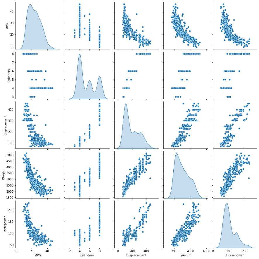
Figure 1: Spark ML pipeline with multiple transformations
To see pairwise correlation of the features we use the heatmap:
corr = mpg_data.corr()
sns.heatmap(corr, annot=True)
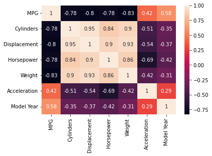
Figure 2: Correlation heatmap
We can see in the scatter plot and correlation matrix that as the horsepower, weight and displacement increase, MPG is reducing.
Build pipeline and transform the data
We will transform only features not the labels. So we split the features and labels in the data:
mpg_data_labels = mpg_data['MPG'].copy().to_numpy()
mpg_data_features = mpg_data.drop('MPG', axis=1)
We will build two pipelines to transform the data. One of the pipeline is for numeric columns which will use these Transformers:
Imputer: Since we have missing values in Horsepower column, we will fill the missing data using median of all the remaining values.
StandardScaler: The features in the dataset are not in the same range. Machine learning algorithms perform well when data is in similar ranges.
We will use StandarScaler to scale the input data.
This pipeline is defined as below:
num_tr_pipeline = Pipeline([
        ('imputer', SimpleImputer(strategy="median")),
        ('std_scaler', StandardScaler()),
    ])
Second pipeline is to transform categorical feature ‘Origin’ to one-hot encoding. This pipeline will have below Transformers:
OrdinalEncoder: Before we convert Origin to a one hot encoding we need to assign label indicies to each unique value. OrdinalEncoder will perform this operation.
OneHotEncoder: Once OrdinalEncoder stage is completed, we can convert the categorical values to one-hot encoding using this transformation.
This pipeline is defined as below:
cat_tr_pipeline = Pipeline([
        ('ordinal_encoder', OrdinalEncoder()),
        ('one_hot_encoder', OneHotEncoder()),
    ])
We need to specify which features should be processed by each pipeline. Since features except Origin are numeric, they should be processed by numeric pipeline.
We define the numeric columns using:
num_attribs = [col for col in mpg_data_features.columns if col != 'Origin']
Origin column should be processed by categorical pipeline. We define the categorical column:
cat_attribs = ['Origin']
Now we can transform the columns using the pipelines:
full_pipeline = ColumnTransformer([
        ("num_tr_pipeline", num_tr_pipeline, num_attribs),
        ("cat_tr_pipeline", cat_tr_pipeline, cat_attribs),
    ])

mpg_transformed = full_pipeline.fit_transform(mpg_data_features)
mpg_transformed will have all the data transformations applied.
Build the model, predict and evaluate the model
Before we build the model, we split the data into train and test data:
mpg_train_data, mpg_test_data, mpg_train_labels, mpg_test_labels = train_test_split(mpg_transformed, mpg_data_labels, test_size=0.3, random_state=0)
First let us try a simple Linear Regression model. Train the model using train data and evaluate how it performs on the test data:
lin_reg = LinearRegression()
lin_reg.fit(mpg_train_data, mpg_train_labels)
mpg_test_predicted = lin_reg.predict(mpg_test_data)
np.sqrt(mean_squared_error(mpg_test_labels, mpg_test_predicted, squared=True))
This gives output of:
3.366034587971452
We will build another model using RandomForestRegressor:
from sklearn.ensemble import RandomForestRegressor

forest_reg = RandomForestRegressor(n_estimators=50, random_state=0)
forest_reg.fit(mpg_train_data, mpg_train_labels)
mpg_test_predicted = forest_reg.predict(mpg_test_data)
np.sqrt(mean_squared_error(mpg_test_predicted, mpg_test_labels, squared=True))
This gives output of:
2.7287667360915995
This is improvement over Linear Regression. We can further tweak the model parameters or build different models to further improve the prediction.
Since the goal of this post was to show the usage of Scikit-Learn ML pipelines, we will stop here.
Complete implementation of Scikit-Learn ML Pipeline for regression
This is available as Jupyter Notebook and as a Python script